Sensor Basics
In this section you will repeat the meaning of basic remote sensing terminology using the example of three satellites which we will continue to use in RESEDA, i.e., Landsat 8, Sentinel 2 and Sentinel 1. However, the shown methods in this online course are also adaptable to other satellite sensors, airborne imagery or close-ups by considering the respective sensor characteristics.
Non-Imaging vs Imaging Sensors
Non-imaging sensors, such as laser profilers or RADAR altimeter, usually provide point data, which do not offer spatially continuous information about how the input varies within the sensor’s field of view.
By contrast, imaging sensors are instruments that build up a spatially continuous digital image within their field of view, whereby they include not only information about the intensity of a given target signal, but also information about its spatial distribution. Examples include aerial photography, visible or near infrared scanner as well as synthetic aperture radars (SAR). All three satellite missions we will work with (Landsat 8, Sentinel 2 and Sentinel 1) are imaging sensors.
Passive vs Active Sensors
Anyway, there is a fundamental differentiation of remote sensing systems that we need to be aware of: passive and active sensors. This classification is based on the underlying recording principles, which are contrasted in the following:
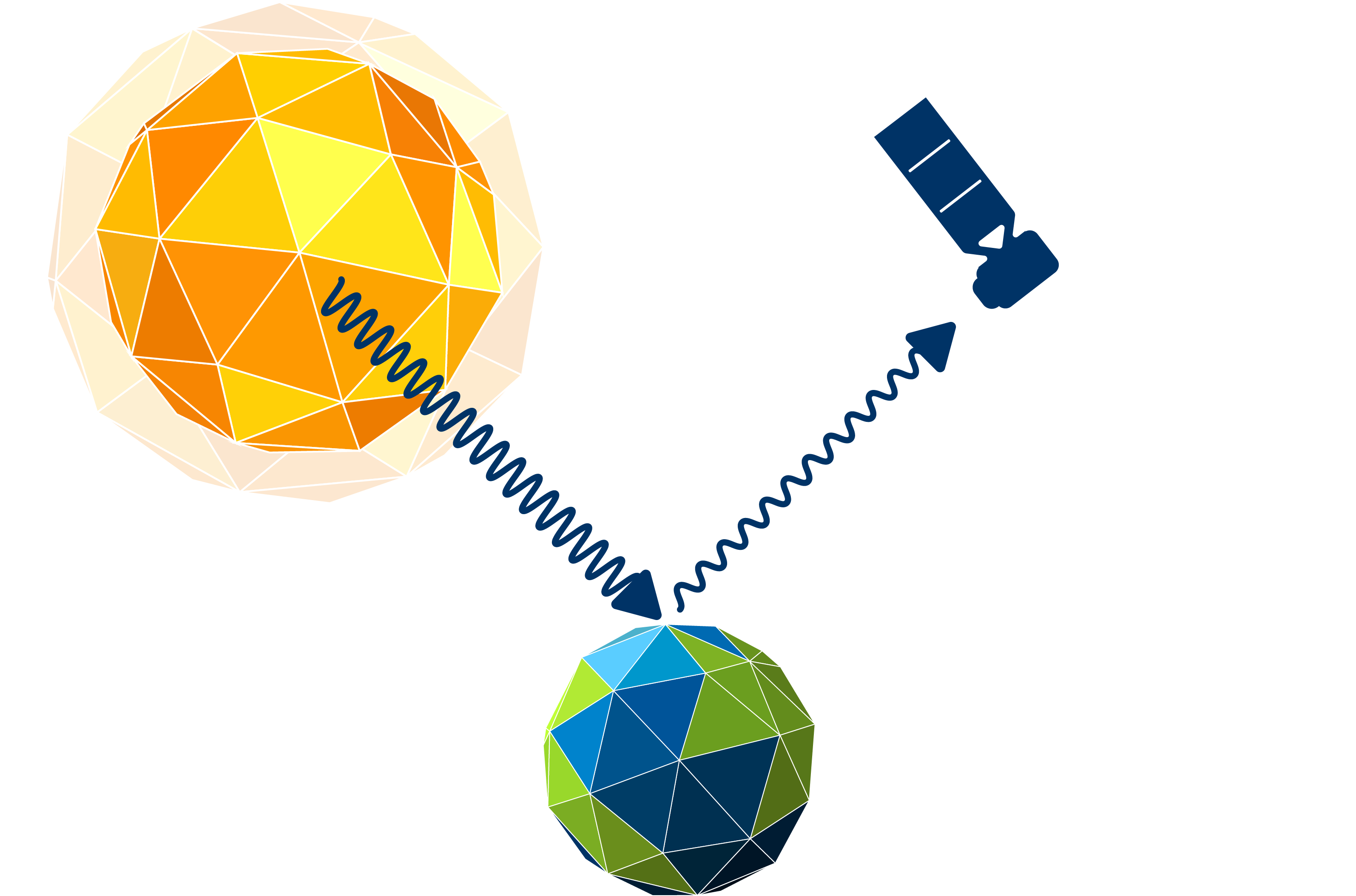
Passive sensor operating mode
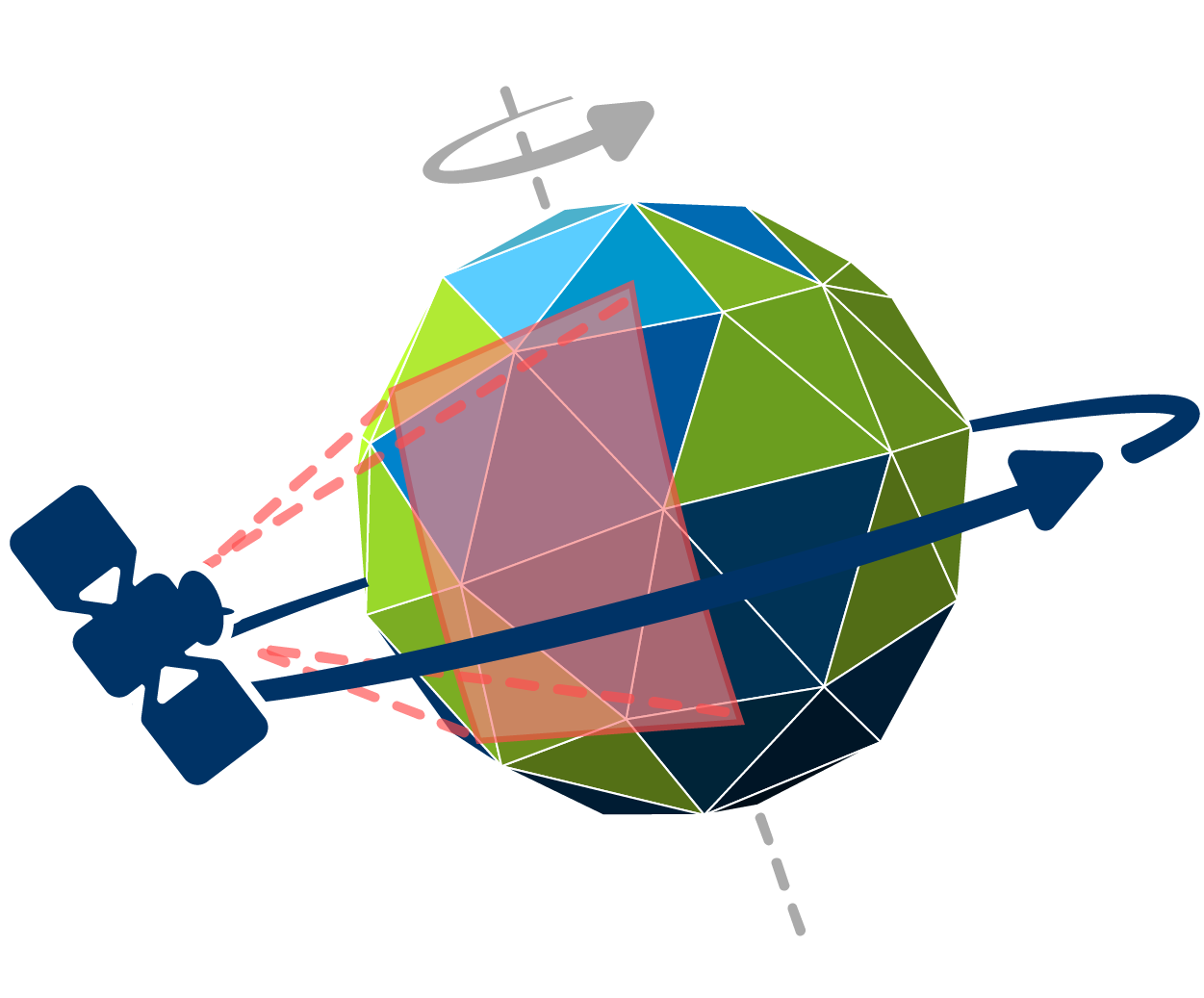
Passive sensors should be the more common of those two. Passive sensors measure solar light reflected or emitted from the Earth surfaces and objects.
These instruments primarily rely on short waved electromagnetic solar energy of the sun as the only source of radiation. Objects on the Earth’s surface react to this electromagnetic energy either with reflection, transmission, or absorption, depending on the composition of the object’s atoms. Passive sensors mainly capture the reflected proportion of the solar energy. Thus, they can only do their observation job when the sun is present as a radiation source – that is, only during the day. Anyway, since objects also partially absorb incoming solar light, there is a inherent radiation of these objects, which can be measured, for example, as thermal radiation.
Passive remote sensing imagery can be very similar to how our human eyes perceive land cover, which makes it easier for us to interpret the image data.
Unfortunately, there is one big limitation of passive systems: Due to the fact that the reflected electromagnetic radiation has to pass through the Earth’s atmosphere, the signal is strongly influenced by the weather and cloud conditions: Fog, haze and clouds render affected image information partially or completely useless, as electromagnetic energy is scattered by the large particles of dense clouds. This is where active sensors come into play.
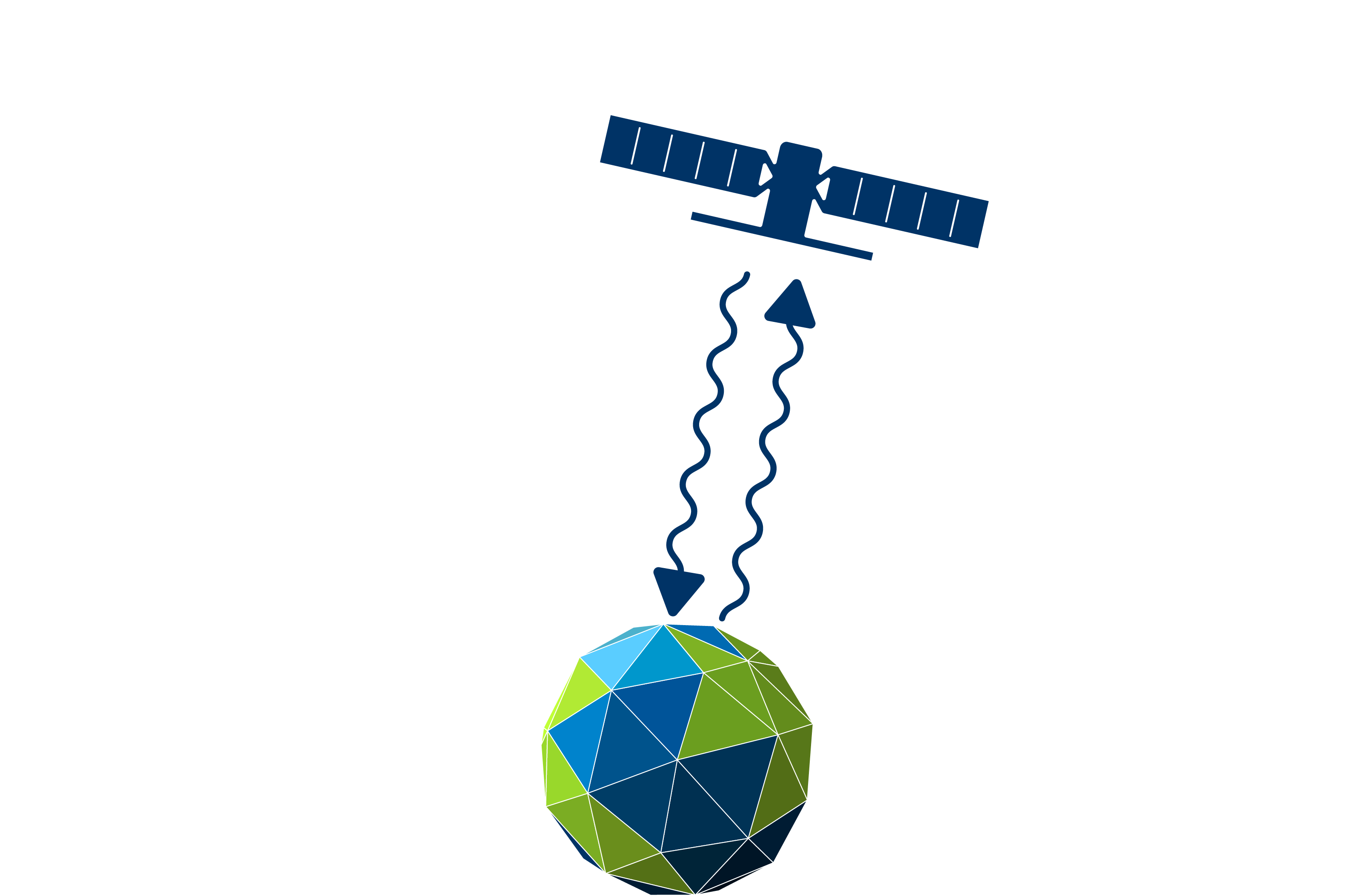
Active sensor operating mode
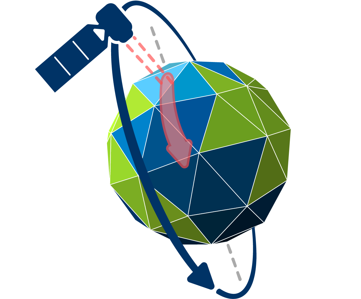
Active sensors emit their own electromagnetic radiation to illuminate the object they observe.
Active sensors send a pulse of energy at the speed of light to the Earth’s surface, that is reflected, refracted or scattered by the objects on the surface and the atmosphere. The recieved backscatter then gives information on land surface characteristics. There are many types of active sensors out there: RADAR (Radio Detection and Ranging), Scatterometer, LiDAR (Light Detection and Ranging), and Laser Altimeter. We will take a closer look at Sentintel 1, a SAR system (Synthetic Aperture RADAR), which is an imaging RADAR type working with microwaves. Images of active sensors are comparatively difficult to interpret: A SAR signal contains amplitude and phase information. Amplitude is the strength of the RADAR response and phase is the fraction of a full sine curve. In order to generate beautiful images out of these information, a more extensive preprocessing is often necessary, which we will do in SNAP.
Since no natural light source is required, active sensors are capable to emit and capture their signals regardless of daytime. In addition, many systems operate in the electromagnetic domain of microwaves, so their wavelength is large enough to be unaffected by clouds and other atmospheric distortions.
Imaging Sensor Resolutions
When working with imaging remote sensing systems, a distinction is made between four different resolution terms: geometric, spectral, radiometric and temporal. It is essential to know those resolutions in order to be able to assess whether the sensor system is suitable for your research question!
1. Geometric Resolution
A digital image consists of at least one matrix of integers values – the picture elements, or pixels. Each pixel contains information about a signal response from a small area on the land surface, e.g., reflectance or backscatter. The geometric Resolution describes the edge length of this area (usually in meters) and is determined by the sensor’s instantaneous field of view (IFOV). It determines which object sizes can still be identified in the image – the degree of detail, so to speak. The effects of geometric resolutions becomes evident when comparing different images, for example an airborne orthophoto (0.1 m), Sentinel 2 (10 m) and Landsat 8 (30 m) images:
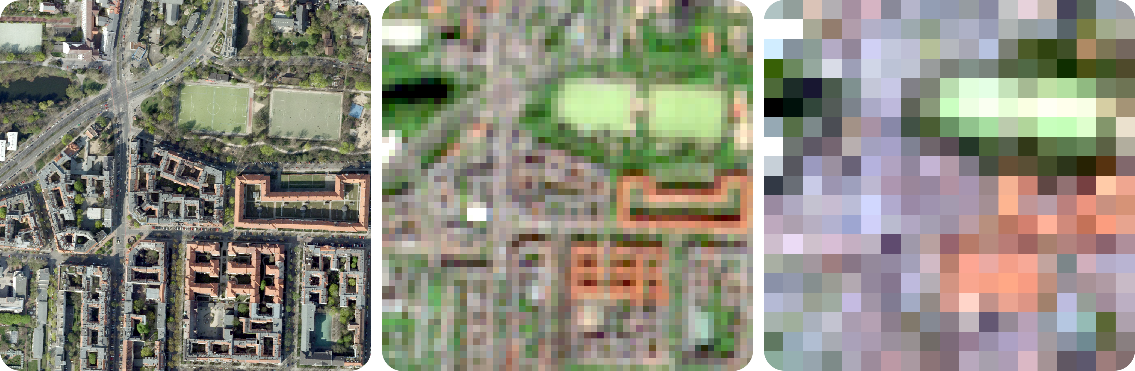
Residential area in Friedenau, orthophoto (l), Sentinel 2 data (m), and Landsat 8 data (r)
There are several synonyms commonly used for the term geometric resolution, e.g., spatial resolution, pixel size, pixel edge length, or ground sampling distance.
2. Spectral Resolution
We humans can only perceive the visible light around us, which is just a very small part of the available electromagnetic spectrum. Satellites, on the other hand, sense a much wider range of the electromagnetic spectrum and can provide us with information about processes that would otherwise be neglected.
Spectral satellite sensors measure the reflection from the earth’s surface in different wavelength areas of the electromagnetic spectrum, via so-called channels or bands. Each band can have a different bandwidth, i.e., the area scanned within the electromagnetic spectrum. The sensors concentrate the signals gathered within a band to one (pixel-) value via a sensor specific filter function.
However, spectral resolution describes the number of bands that the sensor senses. The purpose of multiple bands is to capture the differences in the reflection characteristics of different surfaces and materials within the electromagnetic spectrum.
Panchromatic systems have only one spectral channel with a large bandwidth usually from 0.4 to 0.7 μm. Due to this large bandwidth there is enough energy available to achieve high geometric resolutions. Various satellites additionally provide such a panchromatic channel, e.g., Landsat program, Quickbird-2 pan, and IKONOS pan.
Multispectral systems generally refers to 3 to 15 bands, which are usually located within the visible range (VIS, 0.4-0.7 μm), near-infrared (NIR, 0.75–1.4 μm), short-wavelength infrared (SWIR, 1.4–3 μm), mid-wavelength infrared (MWIR, 3–8 μm) and long wavelength/ thermal infrared (LWIR/TIR, 8–15 μm). Examples: Landsat program, Sentinel 2/3, SPOT, Quickbird, and RapidEye.
Sentinel 2 image, airport Schönefeld, Berlin; left: true color composite (RGB 4,3,2), right: pseudo-color composite (RGB 8,4,3)
Hyperspectral systems (spectrometer) offer hundreds or thousands of bands with narrow bandwidths. A spectral resolution this high gives ability to distinguish minor differences of land cover characteristics, which in turn provides ability to address issues that could not be solved with multispectral data, e.g., mineral or building material classifications. There are some airborne spectrometers (AVIRIS, HySPEX, HyMAP) and to date only one operational satellite: Hyperion. Anyway, more spaceborne systems are already in the starting blocks, e.g., EnMAP and HyspIRI.
3. Radiometric Resolution
A digital sensor generally recognizes objects as intensity values, whereby it can only distinguish between dark and bright. The radiometric resolution refers to the ability to tell apart objects based on differences in those intensities. Thus, a sensor with a high radiometric resolution records more intensity levels or grey-scale levels. This property is expressed by the number of bits. Most satellite products have a bit depth of 8 to 16 bits, which means that they support 28(=256) or 216(=65536) different gray scale levels, respectively. A 1 bit image would be subject to a huge loss of information in comparison!
Those effects are easier to understand when looking at the image comparison below: An image with a bit depth of 1 contains only two gray scale levels (21=2), i.e., black and white. Using 2 bits double the number of available colors (22=4), which allows a few more details (as shown in the middle image). When using 8 bits, the image can draw from a whole color ramp ranging from black to white (dark to bright) comprising 256 grey scale values (28=256).
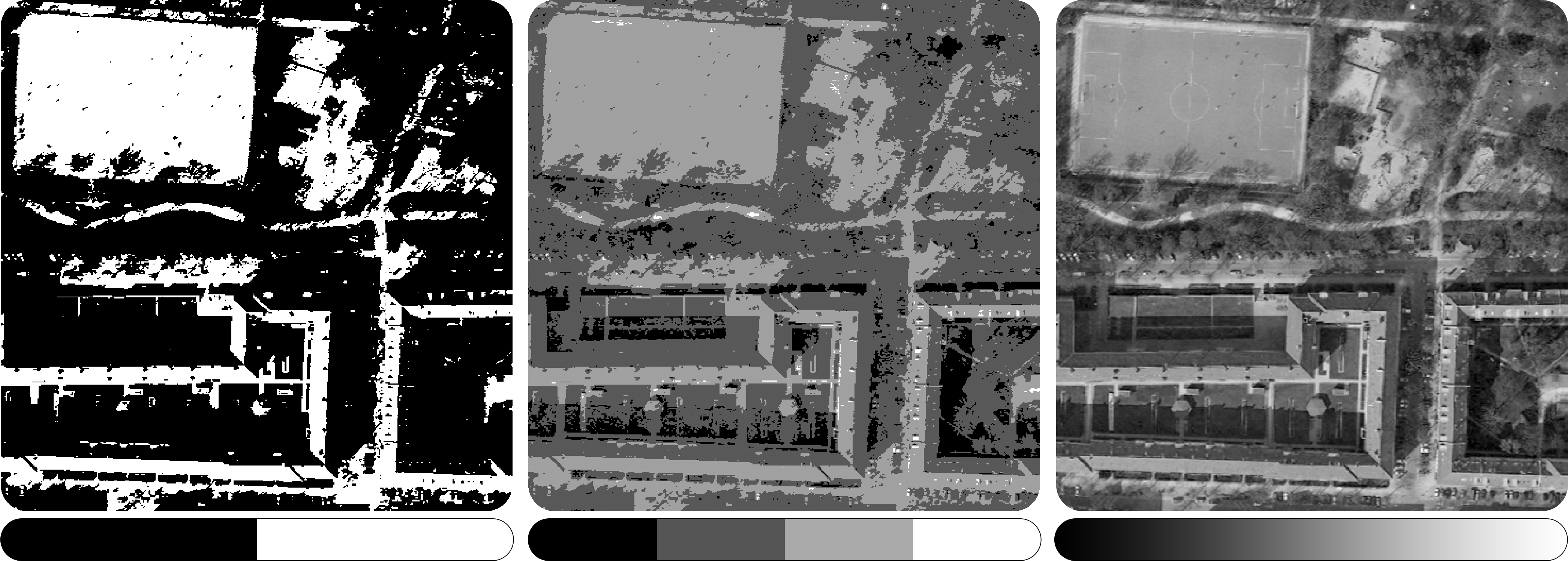
Blue band of an orthophoto in 1 bit (l), 2 bit (m), and 8 bit (r) representation
Human perception is barely sufficient to detect gray-scale differences beyond 8 bits in digital images. Nevertheless, machine learning algorithms often benefit from a finer differentiation of contrasts.
4. Temporal Resolution
The temporal resolution of a sensor is simply the distance of time (usually in days) between two image acquisitions of the same area. A high temporal resolution thus indicates a smaller time window between two images, which allows a better observation of temporally highly dynamic processes on the Earth’s surface, e.g., weather or active fire monitoring.
Most satellite sensors have a temporal resolution of about 14 days. Anyway, by using a satellite constellation of multiple sensors identical in construction the time between two acquisitions can be shortened. For example Planet Labs operates five RapidEye satellites, which are synchronized so that they overlap in coverage.
However, weather satellites are capable of acquiring images of the same area every 15 minutes. This can be explained by the different orbits of the satellites: geostationary and polar orbiting satellite systems.
Geostationary orbiting satellite
Geostationary sensors follow a circular geosynchronous orbit directly above the Earth’s equator. A geosynchronous system provides the same orbital period as the Earth’s rotation period (24 h), so it always looks at the same area on Earth, which it can observate at very high frequencies of several minutes. This rotation pattern is only possible at an altitude very close to 35.786 km, which generally results in a comparatively lower geometric resolution. Geostationary orbits are used by weather, communication and television satellites.
Polar orbiting satellite
Polar orbiting satellites pass above or nearly above the poles on each orbit, so the inclination to the Earth’s equator is very close to 90 degrees. They fly at an altitude of approximately 800-900 km. The lower a satellite flies, the faster it is. That’s why an orbit takes only ~90 minutes. While flying from the north to south pole in 45 minutes, sun-synchronous sensors look at the sunlit side of the Earth (descending images). Moving from south to nord pole results in nighttime imagery (ascending images). On an descending flight, all polar orbiting satellites cross the equator between 10:00 am and 10:15 am (local time) to provide maximum illumination and minimum water vapor to prevent haze and cloud build-up. Due to their inclination, they map the entire surface of the earth within several days (~14 d) as the earth continues to rotate beneath them. The temporal resolution of polar orbiting satellites usually describes the repetition rate at the Equator. The coverage gets better at higher latitudes due to the poleward convergence of the satellite orbits.
Landsat-8 and Landsat-9
Landsat 8 and 9 are the latest installment of the U.S. Landsat satellite series, operated by National Aeronautics and Space Administration (NASA) and United States Geological Survey (USGS). The Landsat program represents the world’s longest continuously acquired collection of spaceborne data in history and since late 2008, all data were made available to all users free of charge.
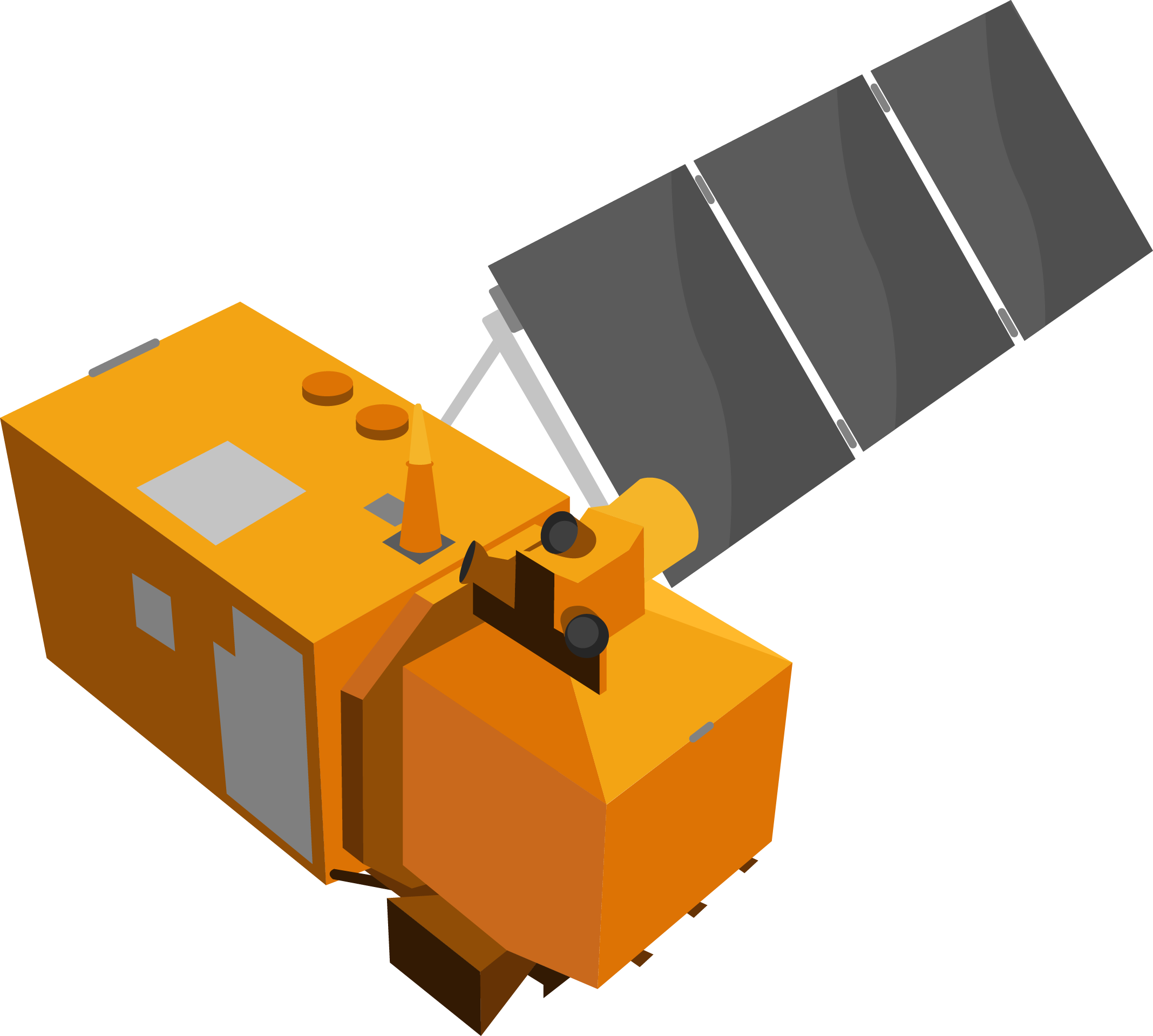
Landsat 8 satellite
The Landsat 8 satellite was launched on February 11, 2013 by an Atlas-V rocket in California, as part of the long-term Earth Observation Systems (EOS) program. Like its predecessors, Landsat 8 is a passive satellite with a multispectral, optical sensor. Landsat 9 was launched September 27th, 2021.
For the first time in the Landsat program, the payload consists of two push-broom instruments onboard – the Operational Land Imager (OLI) and the Thermal Infrared Sensor (TIRS). OLI uses a four-mirror telescope and collects data for visible, near infrared, and short wave infrared spectral bands as well as a panchromatic band. TIRS collects two spectral bands in the thermalinfrared (TIR).
Together, they scan the electromagnetic spectrum in 11 separate bands in a moderate geometric resolutions of 15-30 m:
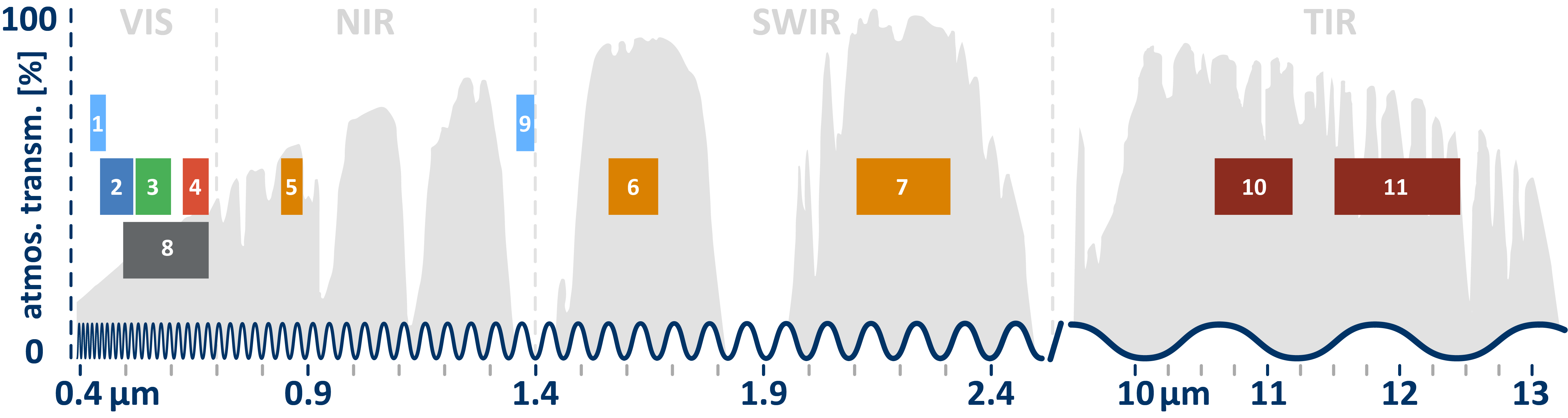
Landsat 8 bands
Each of these channels has been designed to perform certain tasks, e.g., retrieving atmospheric aerosol properties and detect cirrus clouds for corrections of atmospheric distortions (bands 1 & 9), or measuring thermal energy emitted by objects for mapping land surface temperatures (bands 10 & 11):
| BAND | SPECTRAL | WAVELEN. \[µm\] | GEOM. \[m\] | SENSOR |
| 1 | aerosols | 0.435 – 0.451 | 30 | OLI |
| 2 | blue | 0.452 – 0.512 | 30 | OLI |
| 3 | green | 0.533 – 0.590 | 30 | OLI |
| 4 | red | 0.636 – 0.673 | 30 | OLI |
| 5 | NIR | 0.851 – 0.879 | 30 | OLI |
| 6 | SWIR-1 | 1.566 – 1.651 | 30 | OLI |
| 7 | SWIR-2 | 2.107 – 2.294 | 30 | OLI |
| 8 | pan | 0.503 – 0.676 | 15 | OLI |
| 9 | cirrus | 1.363 – 1.384 | 30 | OLI |
| 10 | TIR-1 | 10.600 – 11.190 | 100 | TIRS |
| 11 | TIR-2 | 11.500 – 12.510 | 100 | TIRS |
In the following a profile with the most important characteristics of the sensor is given. For much more detailed information, please refer to the Landsat 8 User Guide and Landsat 9 User Guide!
| geometric |
|
| spectral |
|
| radiometric |
|
| temporal |
|
Data Products
Landsat 8 and 9 each acquire over 500 scenes each day. Most acquired scenes are downlinked to the Landsat Ground Network and made available for download within 24 hours after acquisition. Those scenes are usually uploaded to and stored in the USGS global archive. All Landsat standard data products are processed using the Landsat Product Generation System (LPGS) and come as compressed “.tgz”-files, which can be uncommpressed by using file archiver, such as 7-Zip or WinRAR. Once uncompressed, the image data is in GeoTIFF output format and projected to the Universal Transverse Mercator (UTM) map projection with the World Geodetic System 84 (WGS84) datum.
There are two main data products, which differ in the previous level of preprocessing: one without an atmospheric correction (Level-1) and one with (Level-2). Information on the processing level designations can be found in the metadata file (“.MTL.txt”) that is delivered with the Landsat 8 product.
Level-1 products
Standard Landsat 8 data products consist of quantized and calibrated scaled Digital Numbers (DN) representing the multispectral image acquired by OLI and TIRS. They can be converted to Top Of Atmosphere (TOA) reflectance and radiance values by using radiometric rescaling coefficients as described in this USGS guide.
Level-1 Landsat scenes with the highest available data quality are declared as Tier 1 (L1TP) and are considered suitable for time-series analysis. Tier 1 includes data that have well-characterized radiometry and consistent georegistration and that is inter-calibrated across the different Landsat instruments.
- L1TP (Tier 1): This product offers radiometrically calibrated and orthorectified pixels by using auxiliary digital elevation models (DEM) and ground control points (GCP) to correct for relief displacement
- L1GT (Tier 2): worse, since GCP were not available
- L1GS (Tier 2): worst, since neither GCPs nor DEMs were available
Level-1 products contain the following 14 files once uncompressed:
- Level-1 bands (1, 2, 3, 4, 5, 6, 7, 8, 9, 10 , and 11)
- Quality Assessment (QA) Band
- Angle Band Coefficients file
- Metadata text file (MTL.txt)
Level-2 products
USGS offers on-demand Surface Reflectance data products (Level-2). Surface Reflectance products provide an estimate of the surface spectral reflectance as it would be measured at ground level in the absence of atmospheric scattering or absorption. Surface reflectance values are scaled between 0 % and 100 %. This atmospheric correction is done via the Landsat Surface Reflectance Code (LaSRC), which utilizes the Landsat band 1, auxiliary MODIS data and radiative transfer models.
Keep in mind: This product contain neither Level-1 TOA layers nor thermal bands!
Although these data are also free, it may take several days for the processing to be completed by the servers of the Earth Resources Observation and Science (EROS) Center, before you are able to download them (read on: USGS Earth Explorer).
Level-2 products contain the following 13 files once uncompressed:
Level-2 bands (1, 2, 3, 4, 5, 6, and 7)
Radiometric Saturation QA band (radsat_qa.tif)
Surface Reflectance Aerosol QA band (sr_aerosol.tif)
Level-2 Pixel Quality Assessment band (pixel_qa.tif)
Surface Reflectance metadata file (.xml)
Level-1 metadata file (MTL.txt)
Level-1 Angle Coefficient file (ANG.txt)
In general, we recommend you to use the Level 2 products, especially if you work multitemporally, since the radiometry of surface reflectances is more comparable between scenes.
The official product guide offers more information on the Level-1 and Level-2 Landsat products.
Sentinel-2
Sentinel 2 is a multi-spectral mission consisting of a pair of optical Earth observation satellites: Sentinel-2A and Sentinel-2B, operated by the European Space Agency (ESA) within the framework of the Copernicus program. Sentinel 2 is the European counterpart on Landsat and provides freely available data to study climate change processes.
Sentinel 2 satellite
Both Sentinel 2 satellites were built by Airbus DS and launched on a Vega launch vehicle in French Guiana (Kourou) on June 23, 2015 and on March 7, 2017, respectively. Two more identical satellites are scheduled to launch in 2021 to improve the temporal resolution. Each Sentinel 2 satellite carries a single multi-spectral instrument (MSI), which uses a push-broom concept and provides 13 spectral channels ranging from the visible (VIS) to the short-wavelength infrared (SWIR) in different spatial resolutions. Incoming light is collected by a three-mirror telescope and focused by a beam-splitter onto two focalplane assemblies (FPAs) – one for the ten VNIR bands and one for the three SWIR wavelengths:
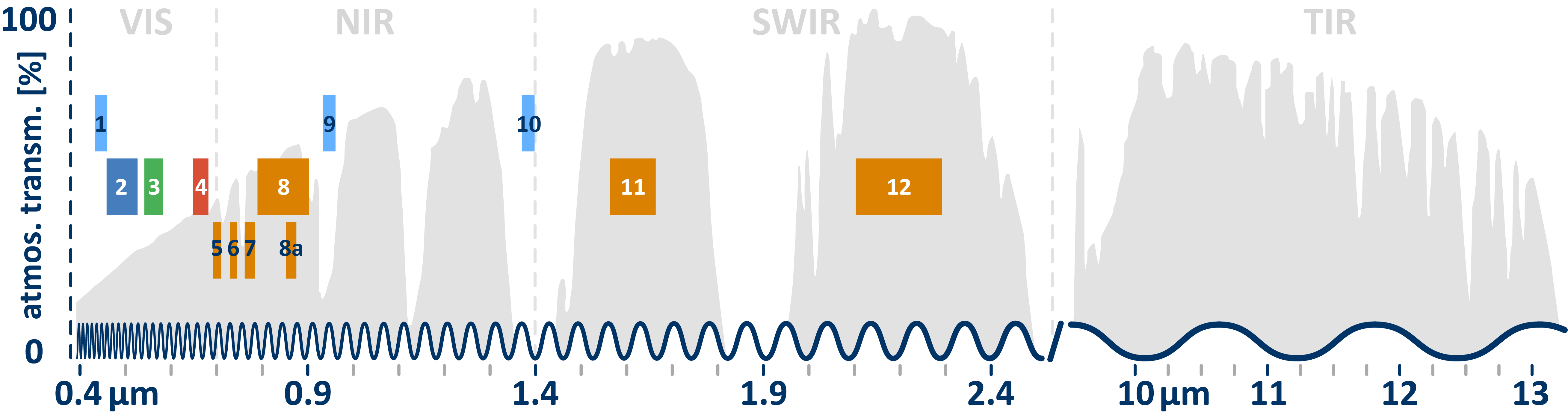
Sentinel 2 bands
The Sentinel 2 mission is designed to mainly provide information for agricultural and forestry practices and applications. In this context, the three red edge bands (5-7) help to differentiate various plant species by leaf area chlorophyll characteristics. Note: Compared to Landsat, however, the thermal and pan bands are missing.
| BAND | SPECTRAL | WAVELEN. \[µm\] | GEOM. \[m\] | SENSOR |
| 1 | aerosols | 0.429 – 0.457 | 60 | MSI |
| 2 | blue | 0.451 – 0.539 | 10 | MSI |
| 3 | green | 0.538 – 0.585 | 10 | MSI |
| 4 | red | 0.641 – 0.689 | 10 | MSI |
| 5 | red edge | 0.695 – 0.715 | 20 | MSI |
| 6 | red edge | 0.731 – 0.749 | 20 | MSI |
| 7 | red edge | 0.769 – 0.797 | 20 | MSI |
| 8 | NIR | 0.784 – 0.900 | 10 | MSI |
| 8a | narrow NIR | 0.855 – 0.875 | 20 | MSI |
| 9 | water vapour | 0.935 – 0.955 | 60 | MSI |
| 10 | SWIR cirrus | 1.365 – 1.385 | 60 | MSI |
| 11 | SWIR | 1.565 – 1.655 | 20 | MSI |
| 12 | SWIR | 2.100 – 2.280 | 20 | MSI |
A special feature of the sensor is the continuous acquisition manner of Sentinel-2, called a “datatake”, which allows a (max.) 15.000 km long continuous imaging strip, e.g. from Russia to southern Africa.
In the following a profile with the most important characteristics of the sensor is given. For much more detailed information, please refer to the Sentinel 2 User Guide!
| geometric |
|
| spectral |
|
| radiometric |
|
| temporal |
|
Data Products
A single Sentinel 2 scene is huge. The swath width of Sentinel 2 is 290 km. So that the data can be handled at all, imagery is geometrically subdivided into rectangular tiles, or so-called granules. The Payload Data Ground Segment (PDGS) is responsible for the processing and archiving those granules. All products are innately projected to the Universal Transverse Mercator (UTM) coordinate system with the World Geodetic System 84 (WGS84) datum.
And again, Sentinel 2 data goes through multiples processing levels:
- Level-0: unprocessed instrument data at full resolution; telemetry analysis, preliminary cloud mask generation, and coarse coregistration
- Level-1A: radiometric corrections and geometric viewing model refinement
- Level-1B: resampling, conversion to reflectances and cloud/water/land mask generation
More information on pre-processing is given in the Sentinel 2 User Handbook.
Anyway, Level-0, Level-1A and Level-1B products are PDGS-internal products not made available to users! When browsing the ESA SciHUB archive, you will be able to choose from Level-1C and Level-2A products:
Level-1C products are radiometric and geometric corrected top of atmosphere (TOA) data. This corrections include orthorectification and spatial registration on the UTM/WGS84 system with sub-pixel accuracy. Level-1C imagary is delivered in granules of 100×100 km of approximately 600-800 MB each. The individual spectral bands are present in their respective resolution (10, 20 and 60m), which is why resampling to a uniform geometric resolution is often necessary for further processing. A product consists of image data, available as JPEG2000 files, and the associated metadata, all capsuled within a “SAFE” file container. You will need the SNAP-software in order to read those SAFE-container (see chapter Visualize for a guide). The Sentinel-SAFE format wraps image data and product metadata in a specific folder structure. Do not alter this folder structure or any file names to ensure that image data and auxiliary information can be imported correctly.
Level-2A is the surface reflectance, or Bottom-Of-Atmosphere (BOA), product derived from a associated Level-1C product. This product is corrected by any distortion of atmosphere, terrain and cirrus clouds. Level-2A datasets come with some additional data layers: aerosol optical thickness-, water vapour, and scene classification maps and quality indicators, including cloud and snow probabilities. You can choose a resolution (10 m, 20 m, or 60 m) in which all channels are resampled uniformly.
Anyway, if you already own a Level-1C scene, the conversion to Level-2A can also be done by yourself via the processor Sen2Cor. A guide on how to do this is given in chapter Classification in R.
In general, we recommend you to use the Level-2A products, especially if you work multitemporally, since the radiometry of surface reflectances is more comparable between scenes.
Sentinel-1
Sentinel 1 is a imaging RADAR mission consisting of a pair of active satellites: Sentinel-1A and Sentinel-1B, operated by the European Space Agency (ESA). Sentinel 1 has initiated the operational phase of Copernicus – the largest European Earth observation program.
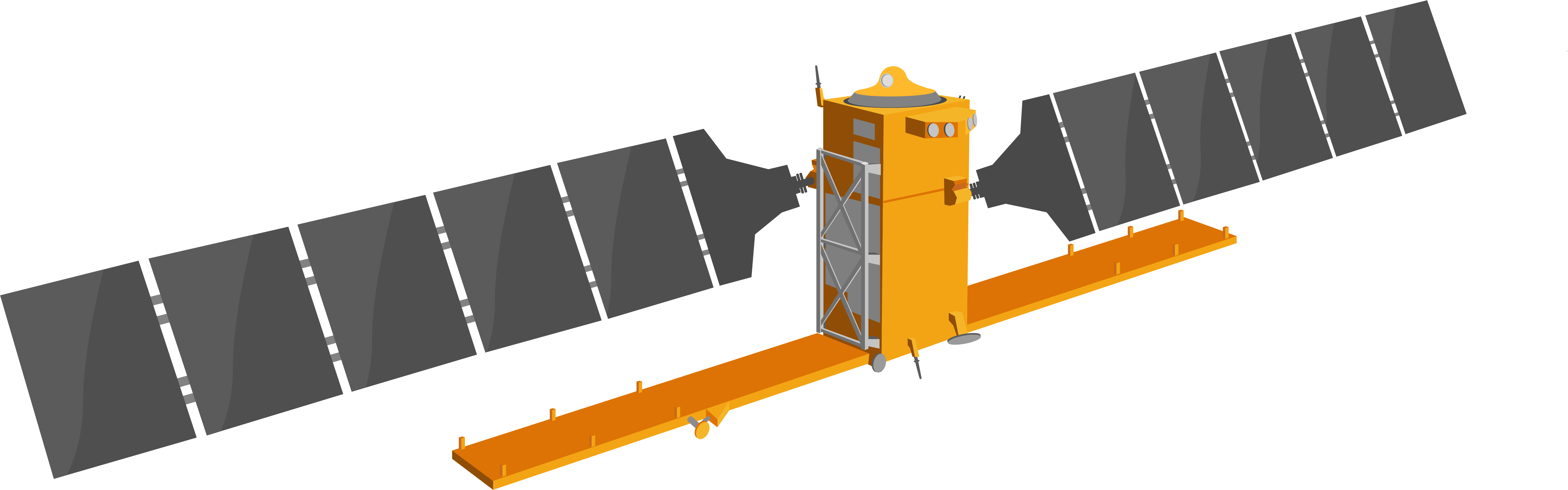
Sentinel 1 satellite
After a seven-year development period led by ESA and Airbus DS, the Sentinel-1A radar satellite was launched on April 3, 2014 with a Russian Soyuz launcher from the European Spaceport Kourou in French Guiana. The identical Sentinel-1B satellite arrived in space two years later, on April 25, 2016. Additionally, Sentinel-1C and 1D are in development with launch dates to be determined.
The main instrument is an imaging C-band SAR (Synthetic Aperture RADAR), consisting of a 12.30 x 0.90 m main antenna composed of 560 single antennas coupled together. Thus, unlike Sentinel 2 or Landsat 8, Sentinel 1 works in the electromagnetic domain of microwaves. It actively emits electromagnetic energy, which has a wavelength of 5.5 cm. The emitted radar rays penetrate through vegetation to the ground. As a result, changes in the surface in the centimeter and even in the millimeter range can be perceived. For a more detailed description of how SAR works.
Sentinel 1 serves a wide range of environmental, transport, economic and security applications. The focus is on ice observation in polar regions, volcanic activity, earthquakes, landslides, floods, detection of subsidence and elevations as well as the observation of sea surfaces to detect issues caused by sea ice and oil spills at an early stage. Furthermore, the satellites are designed to support disaster management in cases of emergency: Wherever up-to-the-minute information is needed, image data can be made available within 60 minutes.
Sentinel 1 has four different observation modes, allowing them to respond to those needs:
- Stripmap (SM): monitor small-scale events upon requests
- Interferometric Wide Swath (IW): primary operation mode for most applications over land
- Extra-Wide Swath (EW): large-scale observation of marine areas
- Wave (WV): primary operational mode over open ocean
According to the ESA Operation Plan the following applications can be mapped to these modes:
| APPLICATION | SM | IW | EW | WV |
| Arctic and sea-ice | ||||
| Open ocean ship surveillance | ||||
| Oil pollution monitoring | ||||
| Marine winds | ||||
| Forestry | ||||
| Agriculture | ||||
| Urban deformation mapping | ||||
| Flood monitoring | ||||
| Earthquake analysis | ||||
| Landslide and volcano monitoring |
Each acquisition mode has different geometrical and therefore different temporal resolution characteristics:
| geometric |
|
| spectral |
|
| radiometric |
|
| temporal |
|
Data Products
Just like Sentinel 2 data, Sentinel 1 ships its data in a zipped “SAFE” container format wrapping image data and product metadata in a specific folder structure. Do not alter this folder structure or any file names to ensure that image data and auxiliary information can be imported correctly. You do not need to unzip the file! The SNAP-software is able to read the file zipped.
Sentinel-1 data products which are generated by the Payload Data Ground Segment (PDGS) operationally are distributed at three levels of processing:
- Level-0: compressed and unfocused SAR raw data, basis for all other high level products
- Level-1: baseline product intended for most data users
- Level-2: geolocated wind, wave and currents products derived from Level-1
For most applications, you should focus on Level-1 data. Additionally, Level-1 products can be one of two product types:
- Single Look Complex (SLC) products are represented by a complex (I and Q) magnitude value and therefore contains both amplitude and phase information
- Ground Range Detected (GRD) products consist of focused SAR data that has been detected, multi-looked and projected to ground range using an Earth ellipsoid model
A more comprehensive explanation of data product is given in the Sentinel 1 user guide.