Regression in R

Very high-resolution reference data are usually difficult to obtain or only available for small areas of the study area. However, low-resolution data, such as Landsat 8 and Landsat 9 (30 m), are available in a high spatio-temporal resolution. Using a regression method, we can create sub-pixel information by relating the high-resolution information to very low-resolution Landsat 9 pixels.

We want to perform a Support Vector Regression in order to regress proportions of imperviousness for each Landsat 9 pixel in Berlin. For this we will use two data sets in this section:

a shapefile containing very high-resolution land cover information (including imperviousness), based on a digitized digital orthophoto of 2016 (Berlin Environmental Atlas)
a Landsat 9 acquisition (ID: LC09_L2SP_193023_20250328_20250329_02_T1), which you may already have acquired during the L8 & L9 Download Exercise

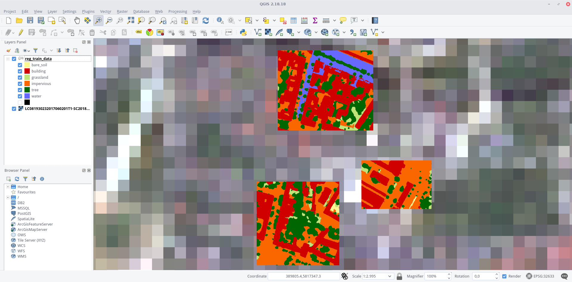
Landsat 8 scene overlaid by the shapefile (colored by classes) in QGIS. The different detail levels become very clear in this visualization

Prepare the samples for training – learn how to preprocess your shapefile
– extract raster features and percentages of your target class (e.g., imperviousness)
– create your training data set for regression analysis
SVM Regression – learn how to perform a Support Vector Regression (SVR) in R using the e1071 package
– predict the whole image data based on your regression model

Prepare Samples for Regression

We want to create training samples in the form of a data frame – which most regressors in R can handle easily. For this we will have to use a few GIS operations. Fortunately, these can also be done automatically in R, so that the entire workflow do not have to be performed manually again and again for other datasets. Finally, we will utilize the terra package for this.

The complete code is shown below. The shapefile reg_train_data.shp and the imagery LC09_L2SP_193023_20250328_20250329_02_T1_subset.tif can be downloaded here.
However, we strongly advise you to have a look at the detailed description in the following.

library(terra)

# Set working directory
setwd("E:\\Work")

# Load the image (Landsat raster) and shapefile
img <- rast("E:\\Work\\LC09_L2SP_193023_20250328_20250329_02_T1_subset.tif")
shp <- vect("E:\\Work\\reg_train_data\\reg_train_data.shp")

# Assign names to raster bands
names(img) <- c("b1", "b2", "b3", "b4", "b5", "b6", "b7")

# Make the shapefile valid (in case it has invalid geometries)
shp <- makeValid(shp)

# Crop image to shapefile extent
img.subset <- crop(img, shp)

# Rasterize the shapefile (covering areas)
img.mask <- rasterize(shp, img.subset, field = 1, cover = TRUE)

# Set all values in img.mask less than 100 to NA
img.mask[img.mask < 100] <- NA

# Mask the image using the created mask
img.subset <- mask(img.subset, img.mask)

# Convert the image to polygons (grid cells)
grid <- as.polygons(img.subset, dissolve = FALSE)

# Add an ID column to grid cells
grid$ID <- seq.int(nrow(grid))

# Create an empty dataframe for storing the results
smp <- data.frame()

# Loop over each grid cell
for (i in 1:nrow(grid)) {
  
  # Get the intersection of the grid cell and the shapefile
  cell <- intersect(grid[i, ], shp)
  
  # Filter for specific classes (e.g., "building" and "impervious")
  cell <- cell[cell$Class_name %in% c("building", "impervious"), ]
  
  if (nrow(cell) > 0) {
    # Calculate the area percentage if there are valid cells
    areaPercent <- sum(expanse(cell) / expanse(grid[i, ]))
    
    # Create the newsmp data frame by combining grid info and area percentage
    newsmp <- cbind(as.data.frame(grid[i, 1:nlyr(img)]), areaPercent)
    
    # Check if newsmp has rows before appending to smp
    if (nrow(newsmp) > 0) {
      smp <- rbind(smp, newsmp)
    }
  }
}

# Display the first few rows of the final dataframe
head(smp)

In-depth Guide

In order to use functionalities of the terra package, load it into your current session via library(). If you do not use our VM, you must first download and install the packages with install.packages():

#install.packages("terra")
library(terra)

Next: set your working directory, in which all your image and shapefile data is stored by giving a character (do not forget the quotation marks " ") variable to setwd(). Check your path with getwd() and the stored files in it via dir():

setwd("E:\\Work")

getwd()
## [1] "E:\\Work"

dir()  
##  [1] "LC09_L2SP_193023_20250328_20250329_02_T1_subset.tif"                                                
##  [2] "reg_train_data.dbf"     
##  [3] "reg_train_data.prj"
##  [4] "reg_train_data.qpj"
##  [5] "reg_train_data.shp" 
##  [6] "reg_train_data.shx"

If you do not get your files listed, there is an error in your working path – check again! Everything ready to go? Fine, then import your raster file as img and your shapefile as shp and have a look at them:

img <- rast("E:\\Work\\LC09_L2SP_193023_20250328_20250329_02_T1_subset.tif")
img
## class       : SpatRaster 
## dimensions  : 504, 1030, 7  (nrow, ncol, nlyr)
## resolution  : 30, 30  (x, y)
## extent      : 369795, 400695, 5812395, 5827515  (xmin, xmax, ymin, ymax)
## coord. ref. : EPSG:32633  (UTM Zone 33N, WGS84)

shp <- vect("E:\\Work\\reg_train_data\\reg_train_data.shp")
shp
## class       : SpatVector 
## geometry    : polygons 
## features    : 286 
## extent      : 390233.4, 390698.4, 5817147, 5817720  (xmin, xmax, ymin, ymax)
## coord. ref. : EPSG:32633 

same.crs <- crs(shp) == crs(img)
print(same.crs) # Should return TRUE if both CRS match

Both the brick() and shapefile() functions are provided by the raster package. As shown above, they create objects of the class RasterBrick and SpatialPolygonsDataFrame respectively. The L8 raster provides 7 bands, and our example shapefile 286 features, i.e., polygons. You can check whether the projections of the two datasets are identical or not by executing compareCRS(shp, img). If this is not the case (output equals FALSE), the raster package will automatically re-project your data on the fly later on. However, we recommend to adjust the projections manually in advance to prevent any future inaccuracies.
Plot your data to make sure everything is imported properly (check Visualize in R for an intro to plotting):

plot(shp)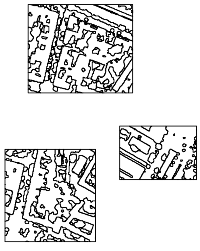

With the argument add = TRUE in line 2 several data layers can be displayed one above the other:

plot(img[[4]], col = gray.colors(100))
plot(shp, add = TRUE, border = "red", lwd = 2)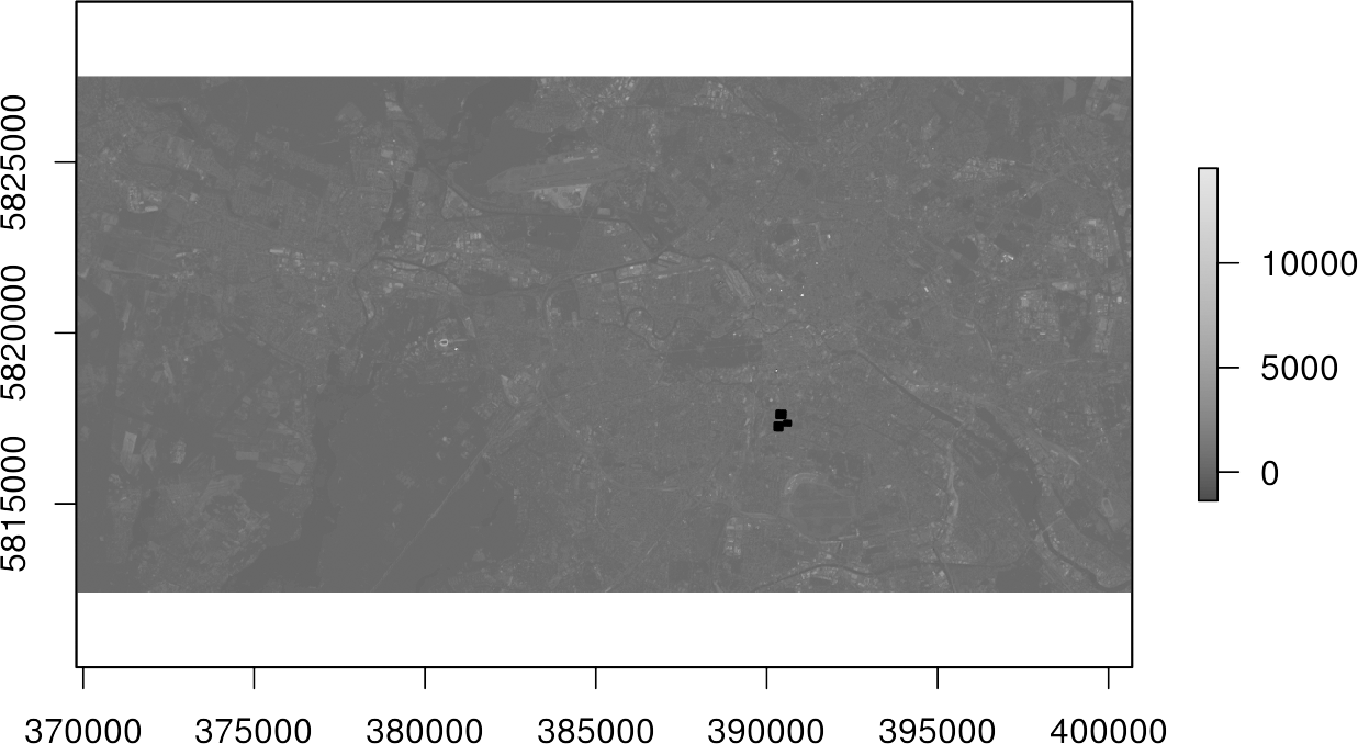

In Line 1, initially only the fourth channel of the image img[[4] was displayed with a gray color representation using 100 shades col=gray.colors(100). The black spots in the upper plot represent the polygons of the shapefile. It becomes clear that they cover only a very small part of our study area.

Optional: Let us take a look at the naming of the raster bands via the names() function. Those names can be quite bulky and cause problems in some illustrations when used as axis labels. You can easily rename it to something more concise by overriding the names with any string vector of the same length:

names(img)
## [1] "LC09_L2SP_193023_20250328_20250329_02_T1_subset.1"
## [2] "LC09_L2SP_193023_20250328_20250329_02_T1_subset.2"
## [3] "LC09_L2SP_193023_20250328_20250329_02_T1_subset.3"
## [4] "LC09_L2SP_193023_20250328_20250329_02_T1_subset.4"
## [5] "LC09_L2SP_193023_20250328_20250329_02_T1_subset.5"
## [6] "LC09_L2SP_193023_20250328_20250329_02_T1_subset.6"
## [7] "LC09_L2SP_193023_20250328_20250329_02_T1_subset.7"

names(img) <- c("b1", "b2", "b3", "b4", "b5", "b6", "b7")

names(img)
## [1] "b1" "b2" "b3" "b4" "b5" "b6" "b7"

In order to accelerate all computation processes in the following, we first trim the image to the extent of the shapefile using the crop() function. It is often recommended to use a buffer of zero width wrapped around the polygons to avoid any topological errors in the upcoming process using gbuffer() as shown in line 1:

shp <- buffer(shp, width = 0)
img.subset <- crop(img, shp)

Now we just want to extract the pixels that are 100% covered by the polygons. Full coverage is important to be able to extract reliable predictions about the ratio of an target class. In order to assess this coverage, we use the rasterize() function with the argument getCover = TRUE to generate a mask. In line 2, we set all pixels which have less than 100% coverage to NA. In the end, we use the mask to subset our image data again using the mask() function:

img.mask <- rasterize(shp, img.subset, field = NULL, touches = TRUE, cover = TRUE)
img.mask[img.mask < 100] <- NA
img.subset <- mask(img.subset, img.mask)

Plot the image data again with the polygons in order to see our achievements:

plot(shp, col = NA, border = "red", lwd = 2)  
plot(img.subset[[4]], add = TRUE)

Only the raster cells within our polygons are left – great!
In a next step, we transform those pixels to polygons, forming a grid with the information of the Landsat 8 bands maintained by using the rasterToPolygons() function. In addition, we want to assign each of these cells in the grid with an ID in order to address them (line 2):

grid <- as.polygons(img.subset)
grid$ID <- 1:nrow(grid)

print(grid)

## class       : SpatialPolygonsDataFrame 
## features    : 93 
## extent      : 390255, 390675, 5817165, 5817705  (xmin, xmax, ymin, ymax)
## coord. ref. : +proj=utm +zone=33 +datum=WGS84 +units=m +no_defs +ellps=WGS84 +towgs84=0,0,0 
## variables   : 8
## names       :   b1,   b2,   b3,   b4,   b5,   b6,   b7, ID 
## min values  :  144,  198,  339,  279,  678,  563,  398,  1 
## max values  : 1175, 1245, 1452, 1422, 3686, 2382, 2193, 93

plot(grid, border = "black", lwd = 0.5)

Finally, we have generated 93 cells (polygons) in this grid for which we now want to make a statement of how much of their areas is impervious, i.e., all polygons that have either building or impervious as Class_name attribute.
For this, we generate a new, empty data frame in which we write the training samples one after the other in line 1. We use a for-loop to iterate over each cell of the grid in line 2:

smp <- data.frame()

for (i in 1:nrow(grid)) {
  
  cell <- intersect(grid[i, ], shp)
  
  cell <- cell[cell$Class_name == "building" | cell$Class_name == "impervious", ]
  
  if (nrow(cell) > 0) {
    areaPercent <- sum(terra::expanse(cell) / terra::expanse(grid[i, ]))
  } else {
    areaPercent <- 0
  }
  
  newsmp <- cbind(as.data.frame(grid[i, 1:nlyr(img)]), areaPercent)
  
  smp <- rbind(smp, newsmp)
}

head(smp)
##      b1   b2   b3   b4   b5   b6  b7  areaPercent
## 2  1175 1245 1452 1422 1742 1321 950 9.765630e-01
## 3   497  597  736  767 1335 1175 947 7.986431e-01
## 5   277  330  477  462 1221  960 743 3.669043e-01
## 4   265  310  444  428 1077  789 545 1.727224e-01
## 41  230  267  390  343  809  613 404 9.765625e-06
## 42  168  217  339  312  678  563 398 3.540961e-02

Explanation:
Line 3: we select the ith cell of the grid and intersect this cell with the shp, which gives us the geometries and attributes of both the shapefile and the cell.
Line 4: only the polygons belonging to the target classes were extracted, we discard all other polygons.
Line 5: if a polygon of a target class exists in the cell, do everything inside the curly brackets. If there is no polygon in the cell, jump to line 7.
Line 6: calculate the proportion of the area of each polygon and sum the proportions ([area(grid)\[1\]equals 900 m² in our example due to the geometric resolution).\ Line 7: if there is no polygon of class *building* or *impervious*, setareaPercentto zero.\ Line 10: use the column bind ([cbind()) function to combine the feature values (reflectances of Landsat image) and the areaPercent value to form a new sample newsmp.
Line 10: use row bind ([rbind()) to add the new samplenewsmpto our training datasetsmp`.

We now prepared a training data set smp with all input features (Landsat 9 bands 1 to 7) and the percentage value of our target class (imperviousness).

Time to train a Support Vector Machine in the next section!

SVM Regression

There are several R packages that provide SVM regression, or Support Vector Regression (SVR), support, e.g., caret, e1071, or kernLab. We will use the e1071 package, as it offers an interface to the well-known libsvm implementation.

Below you can see a complete code implementation. Read the previous section to learn about pre-processing the training data. While this is already executable with the given input data, you should read the in-depth guide in the following to understand the code in detail.

# import
library(terra)
library(e1071)

# Set working directory
setwd("/media/sf_exchange/regression/")

# Load raster and vector data
img <- rast("LC09_L2SP_193023_20250328_20250329_02_T1_subset.tif")
shp <- vect("reg_train_data.shp")

# Rename raster bands
names(img) <- c("b1", "b2", "b3", "b4", "b5", "b6", "b7")

# Crop and mask the raster using the shapefile
img.subset <- crop(img, shp)
img.mask <- rasterize(shp, img.subset, field=1, cover=TRUE)
img.mask[img.mask < 100] <- NA
img.subset <- mask(img.subset, img.mask)

# Convert raster to polygons
grid <- as.polygons(img.subset, dissolve=FALSE)
grid$ID <- seq.int(nrow(grid))

# Prepare training samples
smp <- data.frame()
for (i in 1:length(grid)) {
  cell <- intersect(grid[i, ], shp)
  cell <- subset(cell, Class_name %in% c("building", "impervious"))
  
  if (nrow(cell) > 0) {
    areaPercent <- sum(expanse(cell) / expanse(grid[i, ]))
  } else {
    areaPercent <- 0
  }
  
  newsmp <- cbind(grid[i, 1:nlyr(img)], areaPercent)
  smp <- rbind(smp, newsmp)
}

# Model training
# Define search ranges
gammas <- 2^(-8:3)
costs <- 2^(-5:8)
epsilons <- c(0.1, 0.01, 0.001)

# Start training via grid search
svmgs <- tune(svm,
              train.x = smp[-ncol(smp)],
              train.y = smp[ncol(smp)],
              type = "eps-regression",
              kernel = "radial",
              scale = TRUE,
              ranges = list(gamma = gammas, cost = costs, epsilon = epsilons),
              tunecontrol = tune.control(cross = 5)
)

# Pick best model
svrmodel <- svmgs$best.model

# Use best model for prediction
result <- predict(svrmodel, smp[-ncol(smp)])
result[result < 0] <- 1
result[result < 0] <- 0

In-depth Guide

In order to be able to use the regression functions of the e1071 package, we must additionally load the library into the current session via library(). If you do not use our VM, you must first download and install the packages with install.packages():

#install.packages("terra")
#install.packages("e1071")
library(terra)
library(e1071)

First, it is necessary to process the training samples in the form of a data frame. The necessary steps are shown in line 10-31 and described in detail in the previous section.

After the preprocessing, we can train our Support Vector Regression with the training dataset smp. We will utilize an epsilon Support Vector Regressions, which requires three parameters: one gamma \(\gamma\) value, one cost \(C\) value as well as a epsilon \(\varepsilon\) value (for more details refer to the SVM section). These hyperparameters significantly determine the performance of the model. Finding the best hyparameters is not trivial and the best combination can not be determined in advance. Thus, we try to find the best combination iteratively by trial and error. Therefore, we create three vectors comprising all values that should be tested:

gammas <- 2^(-8:3)
costs <- 2^(-5:8)
epsilons <- c(0.1, 0.01, 0.001)

So we have 14 different values for \(\gamma\), 14 different values for \(C\) and three different values for \(\varepsilon\). Thus, the whole training process is tested for 588 (14 * 14 * 3) models. Conversely, this means that the more parameters we check, the longer the training process takes.
We start the training with the tune() function. We need to specify the training samples as train.x, i.e., all columns of our smp dataframe except the last one, and the corresponding class labels as train.y, i.e. the last column of our smp dataframe, which holds the areaPercentageof our target class imperviousness:

svmgs <- tune(svm,
              train.x = smp[-ncol(smp)],
              train.y = smp[ncol(smp)],
              type = "eps-regression",
              kernel = "radial", 
              scale = TRUE,
              ranges = list(gamma = gammas, cost = costs, epsilon = epsilons),
              tunecontrol = tune.control(cross = 5)
)

We have to set the type of the SVM to "eps-regression" in line 4 in order to perform a regression task. Furthermore, we set the kernel used in training and predicting to a RBF kernel via "radial" (have a look at the SVM section for more details). We set the argument scale to TRUE in order to initiate the z-transformation of our data. The argument ranges in line 7 takes a named list of parameter vectors spanning the sampling range. We put our vectors gammas, costs and epsilons in this list. By using the tunecontrol argument in line 8, you can set k for the k-fold cross validation on the training data, which is necessary to assess the model performance.

Depending on the complexity of the data, this step may take some time. Once completed, you can check the output by calling the resultant object name:

svmgs 
##
## Parameter tuning of ‘svm’:
##
## - sampling method: 5-fold cross validation 
##
## - best parameters:
##       gamma cost epsolon
##  0.00390625    8     0.1
## 
## - best performance: 0.03157376

In the course of the cross-validation, the overall accuracies were compared and the best parameters were determined: In our example, those are 0.0039, 8 and 0.1 for \(\gamma\), \(C\) and \(\varepsilon\), respectively. Furthermore, the Mean Absolute Error (MAE) of the best model is displayed, which is 0.0316, or 3.12%, in our case.

We can extract the best model out of our svmgs to use for image prediction:

svrmodel <- svmgs$best.model
svrmodel 
## 
## Call:
## best.tune(method = svm, train.x = smp[-ncol(smp)], train.y = smp[ncol(smp)], ranges = list(gamma = gammas, cost = costs, 
##     epsolon = epsilons), tunecontrol = tune.control(cross = 5), type = "eps-regression", kernel = "radial", scale = TRUE)
## 
## 
## Parameters:
##    SVM-Type:  eps-regression 
##  SVM-Kernel:  radial 
##        cost:  8 
##       gamma:  0.00390625 
##     epsilon:  0.1 
## 
## 
## Number of Support Vectors:  78

Save the best model by using the save() function. This function saves the model object svrmodel to your working directory, so that you have it permanently stored on your hard drive. If needed, you can load it any time with load().

save(svrmodel, file = "svrmodel.RData")
#load("svrmodel.RData")

Since your SVR model is now completely trained, you can use it to predict all the pixels in your image. The command method predict() takes a lot of work from you: It is recognized that there is an image which will be processed pixel by pixel. As with the training pixels, each image pixel is now individually regressed and finally reassembled into your final regression image. Save the output as raster object result and have a look at its minimum and maximum values (line 11):

result <- predict(img, svrmodel)

result
## class       : RasterLayer 
## dimensions  : 504, 1030, 519120  (nrow, ncol, ncell)
## resolution  : 30, 30  (x, y)
## extent      : 369795, 400695, 5812395, 5827515  (xmin, xmax, ymin, ymax)
## coord. ref. : +proj=utm +zone=33 +datum=WGS84 +units=m +no_defs +ellps=WGS84 +towgs84=0,0,0 
## data source : in memory
## names       : layer 
## values      : -0.7562021, 1.15675  (min, max)

You may will notice some “super-positive” (values above 1.0 or 100%) and/ or some negative (values below 0.0 or 0%) values. Such values are not uncommon, since the SVR implementation of the e1071 package is not subject to any non-negative constraints. You could simply fix this issue by overriding all adequate entries with meaningful minimum and maximum values (0 for 0% and 1 for 100%) by adding the following two lines:

result[result > 1] <- 1
result[result < 0] <- 0

result <- ifel(result > 1, 1, result)
result <- ifel(result < 0, 0, result)

Finally, save your regression raster output using the writeRaster() function and plot your result in R:

writeRaster(result, filename="regression.tif", overwrite=TRUE)

plot(result, col=gray.colors(100))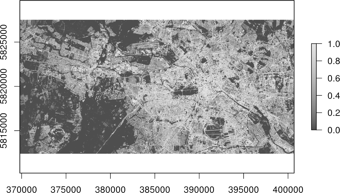

Done! You now got a map, which indicates the percentage of imperviousness, i.e., subpixel-information, for every single pixel in your image data.